Xây dựng mạng CNN phân loại ảnh

CIFAR-10 (Canadian Institute For Advanced Research - 10 classes) là một tập dữ liệu hình ảnh phổ biến được sử dụng trong thị giác máy tính (Computer Vision) và học sâu (Deep Learning). Tập dữ liệu này được phát triển bởi Alex Krizhevsky, Vinod Nair, và Geoffrey Hinton tại University of Toronto và là một trong những benchmark quan trọng để kiểm thử mô hình học sâu. 

Ảnh có kích thước nhỏ (32x32 pixels) nhưng vẫn đủ để huấn luyện các mô hình học sâu. Nó là tập dữ liệu chuẩn, giúp so sánh hiệu suất giữa các mô hình và được sử dụng rộng rãi trong nghiên cứu AI.

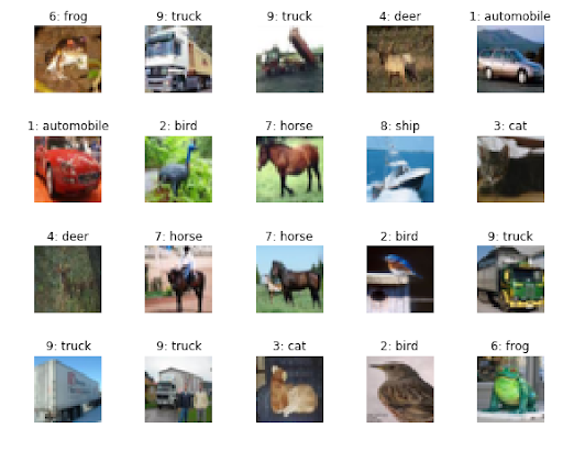
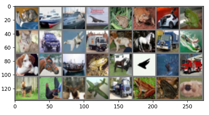
Ảnh 4‑13: Ví dụ hình ảnh của CIFAR-10

Chúng ta sẽ xây dựng một CNN để phân loại ảnh trên tập dữ liệu CIFAR-10, bao gồm 10 loại ảnh như xe cộ, động vật, con người.

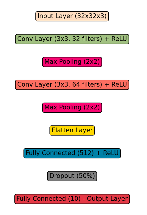
Ảnh 4‑14: Mô hình CNN dùng để huấn luyện nhận biết các lớp

Cài đặt bài toán trên python.

Bước 1: Cài đặt thư viện 

import torch
import torch.nn as nn
import torch.optim as optim
import torchvision
import torchvision.transforms as transforms
import matplotlib.pyplot as plt
import numpy as np

Bước 2: Tải và chuẩn bị dữ liệu CIFAR-10

# Tiền xử lý dữ liệu: Chuyển đổi ảnh thành tensor và chuẩn hóa
transform = transforms.Compose([
    transforms.ToTensor(),
    transforms.Normalize((0.5, 0.5, 0.5), (0.5, 0.5, 0.5))
])
# Tải dữ liệu huấn luyện và kiểm tra
trainset = torchvision.datasets.CIFAR10(root='./data', train=True, download=True, transform=transform)
trainloader = torch.utils.data.DataLoader(trainset, batch_size=32, shuffle=True)
testset = torchvision.datasets.CIFAR10(root='./data', train=False, download=True, transform=transform)
testloader = torch.utils.data.DataLoader(testset, batch_size=32, shuffle=False)

# Các nhãn của CIFAR-10
classes = ('airplane', 'automobile', 'bird', 'cat', 'deer', 'dog', 
           'frog', 'horse', 'ship', 'truck')
# Lấy một batch ảnh từ tập train
dataiter = iter(trainloader)
images, labels = next(dataiter)
# Hiển thị ảnh
def imshow(img):
    img = img / 2 + 0.5  # Bỏ chuẩn hóa
    npimg = img.numpy()
    plt.imshow(np.transpose(npimg, (1, 2, 0)))
    plt.show()
# Hiển thị 4 ảnh đầu tiên trong batch
imshow(torchvision.utils.make_grid(images[:4]))
print(' '.join(classes[labels[j]] for j in range(4)))

Bước 3: xây dựng mô hình CNN

class CNN(nn.Module):
    def __init__(self):
        super(CNN, self).__init__()
        # 1. Lớp tích chập 1: 3 kênh đầu vào (RGB), 32 kênh đầu ra, kernel 3x3
        self.conv1 = nn.Conv2d(in_channels=3, out_channels=32, kernel_size=3, padding=1)
        self.conv2 = nn.Conv2d(32, 64, kernel_size=3, padding=1)
        # 2. Lớp Pooling
        self.pool = nn.MaxPool2d(kernel_size=2, stride=2)
        # 3. Fully Connected Layers
        self.fc1 = nn.Linear(64 * 8 * 8, 512)
        self.fc2 = nn.Linear(512, 10)  # 10 lớp đầu ra
        # Hàm kích hoạt
        self.relu = nn.ReLU()
        self.dropout = nn.Dropout(0.5)
    def forward(self, x):
        x = self.pool(self.relu(self.conv1(x)))  # Conv1 -> ReLU -> MaxPool
        x = self.pool(self.relu(self.conv2(x)))  # Conv2 -> ReLU -> MaxPool
        x = x.view(-1, 64 * 8 * 8)  # Flatten tensor
        x = self.relu(self.fc1(x))  # Fully connected 1
        x = self.dropout(x)  # Dropout để tránh overfitting
        x = self.fc2(x)  # Fully connected 2
        return x
# Khởi tạo mô hình
model = CNN()
print(model)

Bước 4: Định nghĩa hàm mất mát và tối ưu

# Chuyển mô hình sang GPU nếu có
device = torch.device("cuda" if torch.cuda.is_available() else "cpu")
model.to(device)
# Hàm mất mát và bộ tối ưu hóa
criterion = nn.CrossEntropyLoss()
optimizer = optim.Adam(model.parameters(), lr=0.001)
Bước 5: Huấn luyện mô hình
num_epochs = 10  # Số epoch huấn luyện
for epoch in range(num_epochs):
    running_loss = 0.0
    for images, labels in trainloader:
        images, labels = images.to(device), labels.to(device)
        # Forward
        optimizer.zero_grad()
        outputs = model(images)
        loss = criterion(outputs, labels)
        # Backward
        loss.backward()
        optimizer.step()
        running_loss += loss.item()
    print(f"Epoch [{epoch+1}/{num_epochs}], Loss: {running_loss/len(trainloader):.4f}")
print("Huấn luyện hoàn tất!")

Bước 6: Đánh giá mô hình

# Đánh giá trên tập kiểm tra
correct = 0
total = 0
model.eval()  # Đặt mô hình ở chế độ đánh giá
with torch.no_grad():
    for images, labels in testloader:
        images, labels = images.to(device), labels.to(device)
        outputs = model(images)
        _, predicted = torch.max(outputs, 1)
        total += labels.size(0)
        correct += (predicted == labels).sum().item()
accuracy = 100 * correct / total
print(f'Độ chính xác trên tập kiểm tra: {accuracy:.2f}%')

Bước 7: dự đoán một ảnh ngẫu nhiên

# Lấy một ảnh từ tập test
dataiter = iter(testloader)
images, labels = next(dataiter)

# Dự đoán
model.eval()
with torch.no_grad():
    images, labels = images.to(device), labels.to(device)
    outputs = model(images)
    _, predicted = torch.max(outputs, 1)

# Hiển thị ảnh và nhãn dự đoán
imshow(torchvision.utils.make_grid(images.cpu()))
print('Dự đoán:', ' '.join(classes[predicted[j]] for j in range(4)))

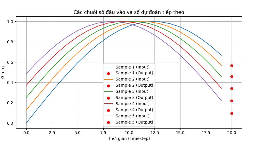
Dưới đây là biểu đồ training của mạng CNN:

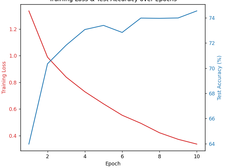
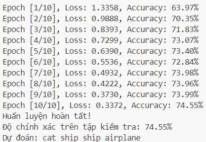
Ảnh 4‑15: Biểu đồ training và kết quả của mạng CNN

Ảnh 4‑16: Dữ liệu trong bộ test để kiểm tra model

Trong kết quả thể hiện 4 ảnh đầu tiên là mèo, tàu, tàu và máy bay.